Porosity and bulk density modelling
Taking a macroscopic approach for the modelling and starting with BD; ρb (g/cm−3) is defined as the total mass of solids (MT) (g) divided by the total volume (VT) (cm−3), ρb = MT/VT where the BD is related to the porosity through the particle density (ρs) of the constituents, φ = 1 − (ρb/ρs). Stewart et al.17 and Adams18 proposed empirical equations equivalent to (Eq. (1)) which we derive physically in the supplementary material (SI Sect. 2.0) using a conservative physical mixing model approach based on mineral and organic constituents:
$${rho }_{b}=frac{1}{frac{SOM}{{rho }_{bOM}}+frac{1-SOM}{{rho }_{bM}}}.$$
(1)
The same form of Eq. (1) is valid for determining the soil particle density18,19 (Eq. S14). Given that φ = 1 − (ρb/ρs) the porosity can be determined:
$$varphi = 1 – left[ {left[ {frac{SOM}{{rho_{sOM} }} + frac{1 – SOM}{{rho_{sM} }}} right] div left[ {frac{SOM}{{rho_{bOM} }} + frac{1 – SOM}{{rho_{bM} }}} right]} right],$$
(2)
where ρsOM and ρsM are the intrinsic particle densities of mineral and organic material. The resulting model requires the values for the SOM, ‘pure’ BD ρOM, ρM and particle density ρsOM, ρsM. According to Ruehlmann and Körschens20 the mean particle density of the soil (ρsoil) can be determined using the particle densities of the SOM and mineral fractions (Eq. S14). They found for the mineral fraction that, ρclay = 2.76 g cm−3; ρsilt = 2.69; ρsand = 2.66; and proposed for the SOM fraction that a dense (ρSOMhd = 1.43 g cm−3) and light (ρSOMld = 1.27) organic fraction could be identified. Where they equate the ρSOMld to the microbial biomass and ρSOMhd to the more dense humified material, for example that occurs in peats and organo-mineral soils. In recent work, Ruehlmann19 collected a comprehensive data set for particle densities of soils for the full range of SOM. We use this data to determine the particle density for our end members in mineral (ρsM 2.7 g cm−3) and organic (ρsOM 1.4 g cm−3) soils (Fig. S1).
Adopting a microscale, or grain scale approach, we are able to exploit recent advances in soft matter physics to gain physical insight into the emergent macro-scale properties21. Studies in soft matter help provide vital understanding into the behavior of granular media. From such studies we know that grain shape, particle size distribution (PSD), repulsion forces and particle friction (µ) are all factors that contribute to the way in which granular media pack22,23. Lattices of spheres have been a source of practical and theoretical interest for millennia. The Kepler conjecture, is perhaps one of the best-known mathematical theorems about 3D mono-size sphere packing. It states that, ‘no packing of congruent balls in Euclidean three-space has density greater than that of the face-centered cubic packing’24. The packing density (η = Vsphere/Vunit cell) or porosity (φ = 1 − η) of lattices of spheres are well known and can be determined mathematically, although the formal proof was only published recently25. They include face centred cubic (π/(3√2) ≈ 0.740 m3 m−3); body centred cubic ((π√3)/8 ≈ 0.680 m3 m−3) and simple cubic (π/6 ≈ 0.524 m3 m−3) for example, with porosity ranging between ~ 0.26 and 0.47 m3 m−3. However, packings of granular media are generally disordered and much more challenging to describe.
Jammed packing’s are used to describe disordered materials, with the ‘maximally jammed random state’ describing the lower bound porosity attainable for mono-size spheres (~ 0.36 m3 m−3)22. Studies of the packing of disordered materials have made substantial progress using computers in soft matter physics, and are largely applicable to the problem of soils, or sediments, which are disordered materials. The problem of determining the porosity of disordered spheres has proved a problem of substantial interest21. Song et al.26 presented a mathematical solution to the problem and composed a phase diagram for the packing of disordered hard spheres. The theory begins by determining the relationship between the free volume of the particle (W) and the geometrical coordination number (z):
$$Wleft(zright)=frac{2sqrt{3}}{z}{text{V}_{g}},$$
(3)
where Vg is the volume of the grains. It shows that W, is inversely related to z. From this starting point they derived an equation of state relating the packing density (η = 1 − φ) to coordination number (z):
$$eta =frac{z}{z+2sqrt{3}}.$$
(4)
They found that for the ground state or maximally jammed random state η = 0.634 for frictionless particles (µ = 0) with z = 6, whereas for the maximally jammed loose state η = 0.591 as µ → ∞ with z = 4. The relationship between packing density and particle friction is presented in Ref.27 with a non-linear relationship. These values correspond well with environmental granular media like sandy soils and sediments (φ ≈ 0.4).
Particle shape orientation and size distribution are also important factors that change the way particles pack22. In this work we incorporate an empirical geometric factor related to shape and acknowledge in our conceptual framework (Fig. S1) that a complimentary model will exist that incorporates particle size, especially where small particles fill the interstices of the large ones. The grain scale approach provides important insight showing that the porosity or BD will depend on characteristics such as the coordination number with other particles, particle shape, size distribution, surface friction and repulsive forces. Moreover, if we combine the macroscale approach (Supplementary Eq. S13) with the microscale approach (Eq. (4)) we can obtain the following equations for mono-size spheres:
$$varphi =frac{2sqrt{3}}{z(mu )+2sqrt{3}},$$
(5)
$${rho }_{b}=frac{{rho }_{s}z(mu )}{z(mu )+2sqrt{3}}.$$
(6)
Further assumptions can be made, for example that 2√3 can be multiplied by an empirical adjustable geometrical factor (2sqrt{3}times GF). By exchanging Eq. (6) into Eq. (1) we obtain new approximations for soil porosity or BD (Eqs. (7), (8)). Where, GF is an empirical geometrical factor > 1 and z is an effective coordination number which, has some power law dependence on the particles friction (µ)27; other symbols are as previously defined:
$$varphi = 1 – left[ {left[ {frac{SOM}{{rho_{sOM} }} + frac{1 – SOM}{{rho_{sM} }}} right] div left[ {frac{SOM}{{frac{{rho_{sOM} zleft( {mu_{OM} } right)}}{{zleft( {mu_{OM} } right) + left( {2sqrt 3 times GF_{OM} } right)}}}} + frac{1 – SOM}{{frac{{rho_{sM} zleft( {mu_{M} } right)}}{{zleft( {mu_{M} } right) + left( {2sqrt 3 times GF_{M} } right)}}}}} right]} right],$$
(7)
$${rho }_{b}=frac{{rho }_{sM}{z({mu }_{M})rho }_{sOM}z({mu }_{OM})}{SOMtimes {rho }_{sM} zleft({mu }_{M}right)left(zleft({mu }_{OM}right)+(2sqrt{3}times {GF}_{OM})right)+{rho }_{sOM}z({mu }_{OM})(-SOM+1)(zleft({mu }_{M}right)times (2sqrt{3}times {GF}_{M}))}.$$
(8)
The result is a set of computationally simple analytical equations that describe the porosity or BD of granular materials with monosize particles that can be adjusted for grain geometry through an empirical geometric factor. Strictly, the models do not include particle size effects that would result in non-conservative mixing and we therefore expect the models to form an upper bound for the physical characteristics of the soil. The contribution of repulsion forces is neglected for temperate, coarse to loamy textured soils, given the wetting and drying cycles resulting in cohesion from suction forces, and organo-mineral particle stabilization. Moreover, data shows that low activity clays, or those with no surface charge such as talc28, produce high porosities (> 0.70 m3 m−3) showing the importance of geometry; we expect counter ions in soils will minimize the effect of electrostatic forces such that geometric factors outweigh electrostatic repulsive forces. Nor do the equations provide insight into the arrangement of the particles, as we point out in our development of conceptual theory and Fig. 2.
National soil data
Figure 3 shows a strong dependence of soil porosity on SOM using a national data set. The data show a clear non-linear change in soil porosity with SOM, modelled with an empirical logarithmic function to show the trend (r2 = 0.81 (actual vs predicted); RMSE = 0.05) (Fig. 3A). Comprehensive national data sets that contain the full range of SOM and BD across land uses are limited, and the lack of samples in soils with higher SOM has prevented previous studies from identifying this trend. The GMEP data set for Wales29 (Fig. 3) offers a comprehensive set of statistically robust topsoil measurements (0–15 cm including SOM and BD) from mineral to organic and for a range of broad habitats. The data clearly show a change in the porosity with the transition across land uses. Porosities are lower for arable (AH) (mean = 0.53 m3 m−3) and improved grassland soils (IG). The broad-leaved woodland (BMYW) (mean = 0.70), neutral (NG) and calcareous (CG) grassland occupy the higher porosities where mineral soils transition to organic. The dashed line represents this transition to organic soils that are occupied by unimproved acid grassland (AG), bracken (Br), coniferous woodland (CW) and dwarf shrub heath (DSH) migrating to the peats in fen march swamp (FMS) and bog (Bo) (mean = 0.91 m3 m−3).
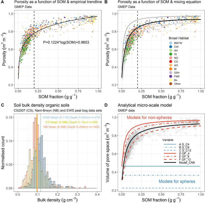
(A) Soil porosity as a function of soil organic matter (SOM) content from the GMEP data set29 n = 1385. An empirical black trendline is fitted to the data (r2 = 0.81 (actual vs predicted); RMSE = 0.05). The dashed line marks the transition from mineral soils (SOM < 0.2) to organic soils (SOM > 0.2). Markers are colour coded by Broad Habitat: broad-leaved woodland (BMYW) coniferous woodland (CW), arable and horticultural (AH), improved (IG), neutral (NG), calcareous (CG) and acid (AG) grassland, bracken (Br), dwarf shrub heath (DSH), fen marsh swamp (FMS) and bog (Bo). (B) The GMEP data set with the black line modelled using Eq. (1) assuming, intrinsic particle densities ρsOM = 1.4 g cm−3 and ρsM = 2.7 g cm−3 and values for the ‘pure’ SOM BD (ρOM = 0.09 g cm−3) and mineral BD (ρM = 1.94 g cm−3). The thick grey line above and the thin grey line below the black line represent approximate bounds based on porosities for mineral granular media13,14 and the standard deviation for the organic soil (SOM > 0.9). (C) Histograms of BD of organic soils from 3 data sets (EWS, UKCEH Countryside Survey and NB Migneint) described in the “Materials and methods”, “Organic soil bulk density data” section, n = 1462. (D) Soil porosity as a function of SOM for the GMEP data set, grey markers. The 3 blue lines are modelled with Eq. (7) assuming spheres with coordination numbers of 4, 6 and 12. The black line is modelled based on Eq. (7) assuming, intrinsic particle densities ρsOM = 1.4 g cm−3 and ρsM = 2.7 g cm−3 and values for (2sqrt{3}times {GF}_{OM}) = 117; zOM = 9 determined by minimizing the sum of squares error; µ is discounted. The red lines represent the same model parameters with the coordination number altered to 4, 6 and 12.
Soil mineral and organic matter conservative mixing model
How well does the macroscale analytical mixing approach (Eqs. (1), (2)) predict porosity? As proposed in the conceptual development Eq. (2) fits the form of the data well when applied to the empirical data in Fig. 3B, anchored by its end members. The black line through the data (Eq. (2)) relies on the following values for the end member intrinsic particle densities ρsOM = 1.4 g cm−3 and ρsM = 2.7 g cm−3. These are determined from Ruehlmann19 as previously described (Fig S1), and values for the ‘pure’ SOM BD (ρbOM = 0.10 g cm−3 ≈ φ = 0.93 m3 m−3) and mineral BD (ρbM = 1.95 g cm−3 ≈ φ = 0.28 m3 m−3). The value of ρbOM is representative of independent values in Fig. 3C. This approach and value are consistent with a number of national data sets presented in Fig. 3C where ~ 2000 measurements in three independent data sets indicate the same approximate value for the BD of mostly uncompact organic soils. The Fig. 3B end points for the porosity of the mineral materials (upper φ = 0.36; lower φ = 0.15 m3 m−3) are taken from Ref.14 for monosize grains (upper) and Ref.13 for the extreme case of clay compressed in sand at a confining pressure of 30 MPa (lower), the value of 0.28 comes from the former for a binary sand mixture. The standard deviation is used to determine the SOM porosities (0.97 and 0.90 m3 m−3). Based on these data and assumptions the model describes the data reasonably well giving a slightly lower fit as expected as it forms an upper bound and is not fitted to the data (r2 = 0.70; RMSE = 0.06). The values are not known a priori and a range of BD values have been presented in the literature, but all from small or incomplete data sets. The BD of organic soils seems to have attracted the least attention in the literature. We consider organic soil and peat independently, with the assumption that peat is likely to represent the organic end member. Perie and Ouimet’s30 organic forest soils resulted in a value of ρOM of 0.111 g cm−3. Whereas, peat soils tend to lie in the range 0.1–0.2 g cm−3 from around the world depending on the degree of humification and compaction31,32. Hence, assuming peat is the end member, we find an average value of ρOM of ~ 0.1 g cm-3 seems appropriate based on the range of evidence for uncompact peat. These results clearly show the dependence of porosity or BD on SOM. Soil formation, environmental, management or degradation factors that lead to changes in SOM will inevitably lead to changes in porosity or BD. Given changes to SOM levels in soils are observed on decadal time scales, we should expect changes in hydraulic function on a similar time scale.
Soil mineral and organic matter mixing model including grain scale
The new porosity (Eq. (7)) and BD (Eq. (8)) models provide an opportunity to explore the data in ways others. In Fig. 3D we apply Eq. (7) to predict porosity (see Fig. S2 for BD), initially with the assumption that all particles are spheres and either mineral or organic (Fig. 3D, straight pale blue lines, A–C). According to the theory of Ref.26 z, should lie between 4 (Fig. 3D, A) and 6 (Fig. 3D, B) for a maximally jammed random state for monosize spheres, while 12 (Fig. 3D, C) is the lower bound for monosize spheres (Face Centred Cubic). Clearly from Fig. 3D the mineral materials with SOM = 0 are approximated by the model, but the organic materials SOM = 1 are not. This is unsurprising as the fibrous nature of peat is hardly spherical. In the next step we maintained the sphere geometry for the mineral component and determined the values for z and (2sqrt{3}times {GF}_{OM}) by fitting the analytical model (Eq. (7)) to the empirical model (Eq. (2), Fig. 3B), assuming the same values for end member intrinsic particle densities ρsOM = 1.4 g cm−3 and ρsM = 2.7 g cm−3. Therefore, the values of z and (2sqrt{3}times {GF}_{OM}) are dependent on the BD of the endpoints and not the data as a whole. The values obtained were 9 for an ‘effective coordination number’ (CN) and 117 for the SOM geometric factor ((2sqrt{3}times {GF}_{OM})), the r2 of the actual vs predicted (fit being r2 = 0.73; RMSE = 0.06). A value of 9 is at the higher end and may be due to mixing of different shapes, or missing physics, such as particle size distribution and repulsion forces23. We then replaced (2sqrt{3}times {GF}_{OM}) with the new empirical value of 117 ((2sqrt{3}times 33.77dots)) and plotted the model predictions for the coordination numbers (CN) of 4 (D), 6 (E) and 12 (F) in Fig. 3D. The modelled data gives a good description for an upper bound to the GMEP data (Fig. 3D). A further independent test was performed by comparing the model (Eq. (7)) with the UKCEH Countryside Survey data which has a much broader spatial coverage and number of habitat locations (n = 2570). The model, without fitting to the data provides a clear, expected, upper bound for the data (Fig. 4).
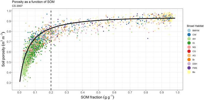
Soil porosity as a function of soil organic matter (SOM) content from the independent UKCEH Countryside Survey 2007 data set36 n = 2570. The dashed line marks the transition from mineral soils (SOM < 0.2) to organic soils (SOM > 0.2). Markers are color coded by Broad Habitat, broad-leaved woodland (BMYW) coniferous woodland (CW), arable and horticultural (AH), improved (IG), neutral (NG), calcareous (CG) and acid (AG) grassland, bracken (Br), dwarf shrub heath (DSH), fen marsh swamp (FMS) and bog (Bo). The black line is the model (Eq. (7)) with CN = 9 and assuming intrinsic particle densities ρsOM = 1.4 g cm−3 and ρsM = 2.7 g cm−3 and values for (2sqrt{3}times {GF}_{OM}) = 117; zOM = 9 as used previously on the GMEP data; µ is discounted.
What do we learn from this new model? The key findings are that the mixing model (Eq. (7)) is an appropriate way to describe an upper bound for the non-linear data (Figs. 3D, 4), but that in order to capture the data fully a non-spherical geometric factor must be applied for the SOM (Fig. 3D, D,GF_4 to F,GF_12). Assuming the model in Fig. 3D is a reasonable approximation of the upper bound, deviation below this could be for a number of physical reasons. Increasing contact resulting from mixing particles of different shapes could partly account for this, as we demonstrate increasing CN to 12. Moreover, particle size, not accounted for in this model, but shown conceptually in Fig. 2 may also account for this reduction in porosity for a given SOM level; while particle arrangement, such as bridging and clustering brought about by friction for example or soil compaction may also play roles. Our results support the observation33 that using the empirical form of the model (Eqs. (1) or (2)) fitted to data will result in a good r2 but with a high RMSE. This high RMSE eludes to the missing physical components not contained in the model, e.g. particle size and compaction for example. Unravelling the complexity to explain the residuals is challenging, but important from both a theoretical point of view, and a practical point of view for prediction. We would also expect that broadening the data set to soils beyond the temperate region, into dryland or low organic matter soils would increase the dominance of particle size for example, as found by others for low SOM soils16,33.
Exploration of the model residuals
Figure 5 explores how soil porosity in different habitats diverges from the analytical model. We use Eq. (7) (Fig. 3D) to explore the residuals as a function of SOM, colored by broad habitat (BH). The porosity residuals plot generated is bounded by the analytical model predictions for different coordination numbers (Eq. (7)). The abscissa corresponds with CN = 9, and the upper grey lines CN = 6 and 4, while the lower darker lines are CN = 12 and 14. The response for each BH and their respective standard deviations are shown by the error bars (see Fig. S3 for the raw scattered data). We would expect that if there is no bias that the soils would be randomly clustered around the zero line (CN = 9). Those exhibiting higher porosity will sit above the line and those with lower will sit below the line. The data shows a clear deviation from the zero line for soils with SOM < 0.2 g g−1 (Fig. 5, Suppl. Fig. S3). These data points represent the managed habitats on mineral soils. The most likely explanation for this is the lack of representation of particle size in the model for mineral soils. The indication that these soils have CN of 12 or greater contact points is only physically feasible if the particle size is greater than monosize. The monosize limit is CN = 12 and only for ordered structures, which is not the case for soils. By plotting the particle size classes on the residual plot (Fig. 6) there does appear to be some of this relationship evident. CN can be determined from the bulk density and SOM by rearranging Eq. (8) to make CN the subject. We used these to determine a median value for CN for each texture class (Supplementary Table S1). The results appear reasonable with sand having the lowest CN values and clay loams and silty clay loams, which have broad PSD, having the highest. The coordination number for sands was 7.3, which compares favorably to measured CN values for natural sands ranging from 6 to 834. Moreover, the CN value increases quickly as sphericity reduces35; in natural beach sand rising from ~ 6 to close to 20 for angular sands. We inserted the appropriate median value of CN into the model for each particle size class. By doing this the r2 and RMSE increased from r2 = 0.73 and RMSE = 0.06 for CN = 9 to r2 = 0.82 and RMSE 0.05 m3 m−3. This is an improvement but highlights that the porosity is a complex interplay between grain shape and size distribution. The dominance of particle shape as a factor over particle size distribution is consistent with other research on physical response, where particle size is a secondary factor, compared to mixing and shape for example, for the electrical properties of porous media like soils14. Moreover, other factors such as rooting, bioturbation and compaction are not accounted for but the high level of variance explained indicates that the major contributing factors in these soils are SOM, particle shape and particle size. These three factors appear to be the dominant characteristics of the soil that determine the emergent nature of soil porosity. However, the relative order of importance will depend on the dominant climatic and soil characteristics. For instance, in drylands with very low SOM particle size and shape are likely to be dominant.
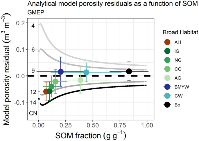
Sensitivity plot for the porosity residuals for the main broad habitats from the model (Eq. (7), black line plotted in Fig. 3D, CN = coordination number) assuming, intrinsic particle densities ρsOM = 1.4 g cm−3 and ρsM = 2.7 g cm−3 and values for the ‘pure’ SOM BD (ρOM = 0.09 g cm−3) and mineral BD (ρM = 1.94 g cm−3) vs SOM. The upper and lower curved lines are the approximate bounds. The solid circle markers represent the mean response by habitat type (Fig. 4 caption) with standard deviation error bars. The highly managed arable (red) and improved grassland (dark green) show the largest deviation from the model.
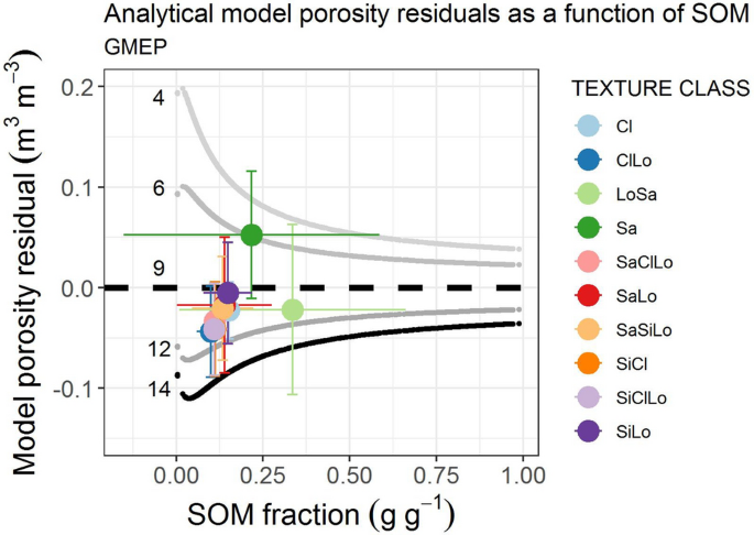
Residuals plotted as a function of SOM for the respective soil texture groups. Markers are color coded by texture class: clay (Cl), clay loam (ClLo), loamy sand (LoSa), sand (Sa), sandy clay loam (SaClLo), sandy loam (SaLo), sandy silty loam (SaSiLo), silty clay (SiCl), silty clay loam (SiClLo), silty loam (SiLo). Median CN values for each texture class shown in Supplementary Table S1. The residuals show a clear particle size effect in the expected direction. The coarse sandy soils having the lowest coordination number and the fine grained clay soils with a broad particle size distribution having the highest CN. This indicates that CN contains both the shape effect and the secondary particle size effect.