In this section, the image dataset for evaluation is introduced first and then the evaluation metrics are described. Extensive comparsion experiments between TSSD algorithm and other methods are carried out in succession. In addition, we give the intuitive discussion about the visual detection effect of this algorithm.
Dataset
In order to verify the effectiveness of the proposed TSSD algorithm, we collect a special dataset of 960 factory smoke images, including 500 captured by mobile phones and 460 downloaded from the Internet. The locations of taking pictures are in different cities, such as Beijing and Zibo, in China. All images contain the chimney, the smoke and the background. These similar things also appear in the Internet pictures. The collected dataset can be divided into four classes according to the image content: sunny environment, cloudy environment, smoke tilting, and multiple chimneys. The examples of the factory smoke dataset are shown in Fig. 5.
The transformation is performed by using Python’s imgaug toolkit. This toolkit can be downloaded from https://github.com /aleju/imgaug. The transformation details for each image are listed below:
(1) Rotate: take the center point of the picture and rotate it. The angle range is from -30 degrees to 30 degrees. According to the affine transformation, each pixel is rotated to the specified position according to the angle; (2) Flip: flip horizontally, mirror, and swap pixels at corresponding positions; (3) Brightness transform: multiply the value of each pixel by the same number, ranging from 0.5 to 1.5. If it is less than 1, it will become dark; otherwise, it will become bright.
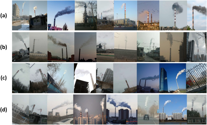
Samples of factory smoke dataset. According to image content, they are divided into four classes of (a–d). Class (a) refers to smoke images in sunny environment. Class (b) corresponds to the cloudy environment. The chimney is inclined in class (c). There are multiple chimneys and smoke zones in class (d).
This dataset is divided according to the training/testing ratio of 7:3, where 672 images act as the training set and the remaining ones as the test. To avoid the over-fitting problem from the few-shot training and learn more essential smoke features by neural networks, we adopt data augmentation strategies to expand the training set and enlarge the diversity of samples, including small-angle rotation, horizontal flip and brightness transform. Using these methods, one factory smoke image can augment to three ones. The details of the dataset distribution are shown in Table 1. The effect of data augmentation is shown in Fig. 6.

Examples of data augmentation. It includes three kinds of augmentation strategies. The first column is the raw data. The second column is to rotate the image, the third is to flip, and the fourth is to transform darkness.
Evaluation metrics
In this paper, the performances of TSSD algorithm and compared methods are evaluated by the following metrics:
Average precision (AP)
We denote the precision rate as P and the recall rate as R. In general, the increase of the precision rate is synchronous with the decrease of the recall rate. To balance them better, PR curve is used to describe the performance of TSSD algorithm. The area under the curve is AP value. Because it’s necessary to locate factory smoke with high accuracy in this research, the AP@IoU(=)0.65:0.05:0.8 is taken as the reference metric. That is marked as AP@65(sim )AP@80.
Mean of different AP values ((AP_{mean}))
To fairly compare TSSD algorithm with mainstream object detection methods, we refer to the evaluation metric36 on the COCO dataset37 and mark the mean of AP@50(sim )AP@95 as (AP_{mean}). It should be noted that this task involves only smoke class.
Inference speed
Model speed is measured by the inference time and FPS (Frames Per Second). The inference time represents the forward time of the neural network detecting one smoke image, while FPS shows the number of the network detecting images per second.
Experimental details
The experimental environment of TSSD algorithm is: in terms of hardware, we adopt the Intel (R) Xeon (R) CPU e5-2660 processor and the graphics card of GeForce RTX 2080 Ti. In terms of software, we choose the Ubuntu 16.04 operating system, TensorFlow1.12.0 deep learning framework, and Python3.6 programming language.
Training details
TSSD algorithm uses the original images and chimney labels as input into the baseline network to train first, which can get a detection model of the chimney. Then, the designed relation-guided module analyses and processes chimney labels to output the reduced smoke detection range. The images of this region and smoke labels are input into the baseline network for training, which can get a smoke detection model. General settings are as follows. The size of network input images is resized to (416times 416). We use a weight decay of 0.0005 and momentum of 0.9, with the batch size of 6 and total epochs of 60. To realize better training effect, we set the initial learning rate as 1e−4 and the termination value as 1e−6, and adopt the warmup strategy to adjust it according to the division of the first 30 epochs and the later epochs.
Testing details
The testing of TSSD algorithm consists of two stages. In the first stage, we use the trained model of chimney detection to output their prediction boxes. In the second stage, we use the designed relation-guided module to carry out the ROI region cropping for the predicted boxes from the previous stage. Then the trained model of smoke predicts the locations of the smoke in this reduced region. The general setting in the test are as follows. The score_threshold of eliminating redundant prediction boxes is 0.6. The size of the network input is (416times 416) except experiments of image resolutions.
Ablation study of TSSD algorithm
This section carries out the ablation study of TSSD algorithm to prove its superiority over the baseline model. In the training process, there are three values worthy to explore: the IoU threshold (varepsilon ) involved in the loss calculation, the balance factor (alpha ) of positive and negative samples, and the hard negative mining coefficient (gamma ). In addition, whether the trained TSSD model can improve the performance on different image resolutions (eta ) is also the discussed problem.
The training IoU threshold (varepsilon )
In order to study the individual effect of the IoU threshold (varepsilon ) on TSSD algorithm, we refer to the best performance of focal loss34 on the COCO dataset and fix the parameter (alpha ) as 0.25 and (gamma ) as 2. In general, the minimum value of (varepsilon ) is set as 0.5 to avoid the big scale of detection boxes involving the loss calculation. What’s more, this paper sets the range of (varepsilon ) as 0.5(sim )0.8, where the step size is 0.1. This aims to compare TSSD with the baseline more fully. The experimental results are shown in Fig. 7.

Comparison of the accuracy between TSSD algorithm and the baseline model at different (varepsilon ) values.
The training balance factor (alpha )
During the training of the baseline network, the proportion of positive and negative samples is 1:10,646. Therefore, it’s of great significance to introduce the balance factor (alpha ) to relieve the loss gap produced by unbalanced two kinds of samples. To explore the performance of TSSD algorithm with different (alpha ) values, we fix (varepsilon ) as 0.5 and (gamma ) as 2. Referring to the setting of (alpha ) in focal loss34, we take it as {0.10,0.25,0.50,0.75}. Fig. 8 shows the experimental results.

Comparison of accuracy between TSSD algorithm and the baseline model at different (alpha ) values.
The training coefficient (gamma )
Introducing the coefficient (gamma ) into the training can reduce the loss influence of simple samples, which enables the neural network to pay more attention to the difficult samples. To verify the performance of TSSD algorithm with different (gamma ) values, we fix (varepsilon ) as 0.50 and (alpha ) as 0.75. In the same way, we refer to the focal loss34 and set (gamma ) as {1,2,4,5}. The experimental results are shown in Fig. 9.

Comparison of accuracy between TSSD algorithm and the baseline model at different (gamma ) values.
The inference image resolution (eta )
Having a good compatibility for different (eta ) inputs is meaningful for TSSD algorithm. Based on the training parameter set of {(varepsilon )=0.5,(alpha )=0.75,(gamma )=2}, we respectively test the (eta ) of (320times 320), (352times 352), and (384times 384). The experimental results are shown in Fig. 10.

Comparison of accuracy between TSSD algorithm and the baseline model at different (eta ) values.
Discussions
From Figs. 7, 8 and 9, it can be clearly seen that TSSD algorithm can steadily improve the detection accuracy of the baseline when to change one of {(varepsilon ), (alpha ), (gamma )} parameters. The conclusion is still valid for different (eta ) sets based on Figure 10. This strongly proves the effectiveness of TSSD algorithm. Especially, from Fig. 7, when to set different (varepsilon ) values, AP@65 and AP@80 of TSSD algorithm can obtain the improvement of over 2(%) and AP@75 over 3(%) than the baseline model. In addition, the biggest gain of 4.45(%) can be got when (varepsilon ) is 0.6 with AP@75. According to Fig. 8, when to set (alpha ) as 0.50 or 0.75, AP@65(sim )AP@75 of TSSD algorithm can increase over 3(%). Moreover, the highest increase of 5.09(%) appears at (alpha ) as 0.50 with AP@70. On the basis of Fig. 9, for all the mentioned (gamma ) parameter settings, AP@75 of TSSD algorithm can realize the raise of over 3 (%) and AP@80 over 2(%). Meanwhile, the best raise occurs at (gamma ) as 5 with AP@75. In Table 2, when (eta ) is (320times 320) or (384times 384), AP@75 and AP@80 of TSSD algorithm can increase over 3(%), and AP@65(sim )AP@80 gets the gain of over 2(%) at (eta ) as (352times 352).
TSSD algorithm realizes so outstanding performance on different training parameters and we think there are three reasons as follows. (1) The relation-guided module in TSSD algorithm can transform the range of detection from the global ROI to the local ROI, which undoubtedly reduces the searching space of the needed object. This helps the neural network achieve more accurate regression for the object’s bounding boxes, determining the finer location of the object. (2) Prior knowledge information is introduced into TSSD algorithm, so that the reduced-range images must contain the smoke object, which improves the certainty of object detection. (3) The relation-guided module effectively eliminates the interference of the objects similar to smoke outside the reduced region.
In addition, by resizing to change (eta ), it only has a certain influence on the clarity of images. That doesn’t damage the inherent location relation between the smoke and the chimney. In other words, the optimization strategy of TSSD algorithm stills works and is not affected.
Comparison with the state-of-the-art detection methods
To verify the comprehensive performance of TSSD algorithm, we compared it with various state-of-the-art detection methods, including Faster RCNN17, SSD18 and the baseline model. For Faster RCNN, we choose Resnet50 and Resnet10138 as the feature extraction networks. For SSD, we use Inception-v239 and MobileNet-v240.
To fairly compare all the models, the size of the network input is set as (416times 416), and their training is based on the pre-trained weight on the COCO. Faster RCNN and SSD are trained until the loss function converges with the stable accuracy. The baseline model and TSSD algorithm adopt the same training parameter settings {(varepsilon )=0.5,(alpha )=0.75,(gamma )=2}. For the fair evaluation between these models, we choose (AP_{mean}) as the accuracy metric. The experimental results are shown in Table 2, where the inference speed of TSSD algorithm is the time sum of the two stages. The effectiveness of it is intuitively visualized in Fig. 11.

Visual effect of TSSD algorithm on detecting factory smoke.Four-class smoke images of dataset are all included. Blue boxes represent the reduced detection range, and red boxes show the detected smoke region. The text on top of each bounding box represents the confidence of smoke detection.
From Table 2, it’s known that the detection accuracy of TSSD model is 59.24(%). It reaches the highest accuracy, even surpassing the current detection model Faster RCNN101. Although TSSD model is slower than the fastest model SSD_Mobilenet-v2, it has the accuracy improvement of 8.42(%). Meanwhile, the speed of TSSD model is 50 ms (20 FPS), meeting the need of real-time detection. All of these show that our proposed TSSD algorithm has a bigger advantage than other methods.
We think there are two primary reasons for such superiority. (1) The baseline model of TSSD algorithm is suitable for this task. Its detection accuracy is only 1.6(%) lower than Faster RCNN_Resnet101, but the speed is 3.25 times faster. Although the speed is slightly slower than SSD_Mobilenet-V2, its accuracy is 6.34(%) higher. (2) The TSSD can robustly improve the accuracy of the baseline model. The specific reasons can be seen in “Ablation Study of TSSD algorithm”.