We define ten research questions to provide a framework for the study. The first group of questions revolves around coding practices (RQ 1–3), while the other around the automated code re-execution (RQ 4–10).
RQ 1. What are the basic properties of a replication package in terms of its size and content?
Our first research question focuses on the basic dataset properties, such as its size and content. The average size of a dataset is 92 MB (with a median of 3.2 MB), while the average number of files in a dataset is 17 files (the median is 8). Even though it may seem that there is a large variety between datasets, by looking at the distributions, we observe that most of the datasets amount to less than 10 MB (Fig. 3a) and contain less than 15 files (Fig. 3b).

Dataset sizes and file counts.
Analyzing the content of replication packages, we find that about 40% of them (669 out of 2,091) contain code in other programming languages (i.e., not R). Out of 2091 datasets, 620 contained Stata code (.do files), 46 had Python code (.py files), and 9, 7, and 6 had SAS, C++, and MATLAB code files, respectively. The presence of different programming languages can be interpreted in multiple ways. It might be that a dataset resulted in a collaboration of members who preferred different languages, i.e., one used R and another Stata. Alternatively, it may be that different analysis steps are seamlessly done in different languages, for example, data wrangling in R and visualization in Python. However, using multiple programming languages may hinder reproducibility, as an external user would need to obtain all necessary software to re-execute the analysis. Therefore, in the re-execution stage of our study, it is reasonable to expect that replication packages with only R code would perform better than those with multiple programming languages (where R code might depend on the successful execution of the code in other languages).
The use of R Markdown and Rnw have been encouraged to facilitate result communication and transparency10. R Markdown (Rmd) files combine formatted plain text and R code that provide a narration of research results and facilitate their reproducibility. Ideally, a single command can execute the code in an R Markdown file to reproduce reported results. Similarly, Rnw (or Sweave) files combine content such as R code, outputs, and graphics within a document. We observe that only a small fraction of datasets contain R Markdown (3.11%) and Rnw files (0.24%), meaning that to date few researchers have employed these methods.
Last, we observe that 91% of the files are encoded in ASCII and about 5% in UTF-8. The rest use other encodings, with ISO-885901 and Windows-1252 being the most popular (about 3.5% together). In the code cleaning step, all non-ASCII code files (692 out of 8173) were converted into ASCII to reduce the chance of encoding error. In principle, less popular encoding formats are known to sometimes cause problems, so using ASCII and UTF-8 encoding is often advised11.
RQ 2. Does the research code comply with literate programming and software best practices?
There is a surge of literature on best coding practices and literate programming12,13,14,15,16 meant to help developers create quality code. One can achieve higher productivity, easier code reuse, and extensibility by following the guidelines, which are typically general and language agnostic. In this research question, we aim to assess the use of best practices and programming literacy in the following three aspects: meaningful file and variable naming, presence of comments and documentation, and code modularity through the use of functions and classes.
Best practices include creating descriptive file names and documentation. Indeed, if file names are long and descriptive, it is more likely that they will be understandable to an external researcher. The same goes for additional documentation within the dataset. We observe that the average filename length is 17 characters without the file extension, while the median is 16. The filename length distribution (Fig. 4a) shows that most file lengths are between 10 and 20 characters. However, we note that about a third or 32% (669) of file names contain a’space’ character, which is discouraged as it may hinder its manipulation when working from the command line. We also searched for a documentation file, or a file that contains “readme”, “codebook”, “documentation” “guide” and “instruction” in its name, and found it in 57% of the datasets (Fig. 4b). The authors may have also adopted a different convention to name their documentation material. Therefore, we can conclude that the majority of authors upload some form of documentation alongside their code.
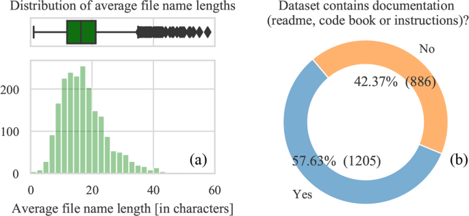
File name lengths and presence of documentation.
Further, we examine the code of the 8875 R files included in this study. The average number of code lines per file is 312 (the median is 160) (Fig. 5a). Considering that there are typically 2 R files per dataset (median, mean is 4), we can approximate that behind each published dataset lies about 320 R code lines.
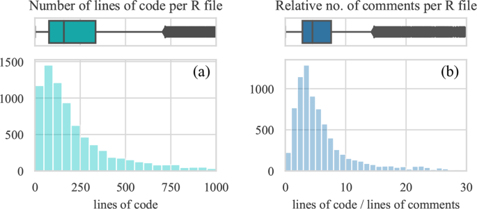
Number of code line and relative number of comments.
Comments are a frequent part of code that can document its processes or provide other useful information. However, sometimes they can be redundant or even misleading to a reuser. It is good practice to minimize the number of comments not to clutter the code and replace them with intuitive names for functions and variables12. To learn about commenting practices in the research code, we measure the ratio of code lines and comment lines for each R file. The median value of 4.5 (average is 7) can be interpreted as one line of comments documenting 4 or 5 lines of code (Fig. 5b). In other words, we observe that comments comprise about 20% of the shared code. Though the optimal amount of comments depends on the use case, a reasonable amount is about 10%, meaning that the code from Harvard Dataverse is on average commented twice as much.
According to IBM studies, intuitive variable naming contributes more to code readability than comments, or for that matter, any other factor14. The primary purpose of variable naming is to describe its use and content, therefore, they should not be single characters or acronyms but words or phrases. For this study, we extracted variable names from the code using the built-in R function ls(). Out of 3070 R files, we find that 621 use variables that are one or two characters long. However, the average length of variable names is 10, which is a positive finding as such a name could contain one, two, or more English words and be sufficiently descriptive to a reuser.
Modular programming is an approach where the code is divided into sections or modules that execute one aspect of its functionality. Each module can then be debugged, understood, and reused independently. In R programming, these modules can be implemented as functions or classes. We count the occurrences of user-defined functions and classes in R files to learn how researchers structure their code.
Out of 8875 R files, 2934 files have either functions or classes. Applying a relative number of modules per lines of code, we can estimate that one function on average contains 82 lines of code (mode is 55). According to a synthesis of interviews with top software engineers, a function should include about 10 lines of code12. However, as noted in Section 0, R behaves like a command language in many ways, which does not inherently require users to create modules, such as functions and classes. Along these same lines, R programmers do not usually refer to their code collectively as a program but rather as a script, and it is often not written with reuse in mind.
RQ 3. What are the most used R libraries?
The number of code dependencies affects the chances of reusing the code, as all dependencies (of adequate versions) need to be present for its successful execution. Therefore, a higher number of dependencies can lower the chances of their successful installation and ultimately code re-execution and reuse. We find that most datasets explicitly depend on up to 10 external libraries (Fig. 6) with individual R files requiring an average of 4.3 external dependencies (i.e., R libraries). The dependencies in code were detected by looking for “library”, “install.packages” and “require” functions.
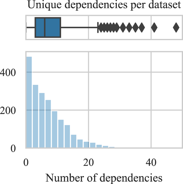
Distribution of unique dependencies per dataset.
The list of used libraries provides insight into the goals of research code (Fig. 7). Across all of the datasets, the most frequently used library is ggplot2 for plotting, indicating that the most common task is data visualization. Another notable library is xtable, which offers functions for managing and displaying data in a tabular form, and similarly provides data visualization. Many libraries among the top ten are used to import and manage data, such as foreign, dplyr, plyr and reshape2. Finally, some of them are used for statistical analysis, like stargazer, MASS, lmetest and car. These libraries represent the core activities in R: managing and formatting data, analyzing it, and producing visualizations and tables to communicate results. The preservation of these packages is, therefore, crucial for reproducibility efforts.
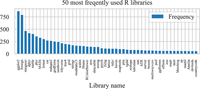
Most frequently used R libraries.
The infrequent usage and absence of libraries also tell us what researchers are not doing in their projects. In particular, libraries that are used for code testing, such as runit, testthat, tinytest and unitizer, were not present. Although these libraries are primarily used to test other libraries, they could also confirm that data analysis code works as expected. For example, tests of user-defined functions, such as data import or figure rendering, could be implemented using these libraries. Another approach that can aid in result validation and facilitate reproducibility is computational provenance17,18. It refers to tracking data transformations with specialized R libraries, such as provR, provenance, RDTlite, provTraceR. However, in our study, we have not found a single use of these provenance libraries. In addition, libraries for runtime environment and workflow management are also notably absent. Libraries such as renv, packrat and pacman aid in the runtime environment management, and workflow libraries, such as workflowR, workflows, and drake provide explicit methods for reproducibility and workflow optimization (e.g., via caching and resource scaling). None of these were detected in our dataset, except for renv which was used in 2 replication packages. Though we can conclude that these approaches are not currently intuitive for the researchers, encouraging their use could significantly improve research reproducibility and reuse.
Finally, we look for configuration files used to build a runtime environment and install code dependencies. One of the common examples of a Python configuration file is requirements.txt, though several other options exist. For a research package (compendium), a DESCRIPTION configuration file that captures project metadata and dependencies was proposed19. We find 9 out of 2091 replication packages that have a DESCRIPTION file and 30 where the word description is contained in any of the file names. Another more Python-ic approach to the environment capture is saving dependencies in a configuration file named install.R. We have not found a single install.R among the analyzed datasets, but we found similar files such as: installrequirements.R, 000install.R, packageinstallation.R or postinstall. Our results suggest that the research community that uses Harvard Dataverse does not comply with these conventions, and one reason for that may be its recent emergence as the publication was released in 2018 (before that, a DESCRIPTION file was typically used for R libraries). Finally, a R user may use the library packrat or renv or a built-in function sessionInfo() to capture the local environment. We have not found any files named ‘sessionInfo’, but we found four packages containing .lock files (two of those called renv.lock) used in the renv library.
RQ 4. What is the code re-execution rate?
We re-executed R code from each of the replication packages using three R software versions, R 3.2, R 3.6, and R 4.0, in a clean environment. The possible re-execution outcomes for each file can be a “success”, an error, and a time limit exceeded (TLE). TLE occurs when the time allocated for file re-execution is exceeded. We allocated up to 5 hours of execution time to each replication package, and within that time, we allocated up to 1 hour to each R file. The execution time may include installing libraries or external data download if those are specified in the code. The replication packages that have resulted in TLE were excluded from the study, as they may have eventually executed properly with more time (some would take days or weeks). To analyze the success rate of the analysis, we interpret and combine the results from the three R versions in the following manner (illustrated in Table 1):
-
1.
If there is a “success” one or more times, we consider the re-execution to be successful. In practice, this means that we have identified a version of R able to re-execute a given R file.
-
2.
If we have one or more “TLE” and no “success”, the combined result is a TLE. The file is then excluded to avoid misclassifying a script that may have executed if given more time.
-
3.
Finally, if we have an “error” 3 times, we consider the combined results to be an error.
We re-execute R code in two different runs, with and without code cleaning, using in each three different R software versions. We note that while 9078 R files were detected in 2109 datasets, not all of them got assigned a result. Sometimes R files exceeded the allocated time, leaving no time for the rest of the files to execute. When we combine the results based on the Table 1, we get the following results in each of the runs:
| Without code cleaning | With code cleaning | Best of both | |
| Success rate | 25% | 40% | 56% |
| Success | 952 | 1472 | 1581 |
| Error | 2878 | 2223 | 1238 |
| TLE | 3829 | 3719 | 5790 |
| Total files | 7659 | 7414 | 8609 |
| Total datasets | 2071 | 2085 | 2109 |
Going forward, we consider the results with code cleaning as primary and further analyze them unless different is stated.
RQ 5. Can automatic code cleaning with small changes to the code aid in its re-execution?
To determine the effects of the code cleaning algorithm (described in Section 4), we first re-execute original researchers’ code in a clean environment. Second, we re-execute the code after it was modified in the code-cleaning step. We find an increase in the success rate for all R versions, with a total increase of about 10% in the combined results (where only explicit errors and successes were recorded, and TLE values were excluded).
Looking at the breakdown of coding errors in Fig. 8, we see that code cleaning can successfully address some errors. In particular, it fixed all errors related to the command setwd that sets a working directory and is commonly used in R. Another significant jump in the re-execution rate results from resolving the errors that relate to the used libraries. Our code cleaning algorithm does not pre-install the detected libraries but instead modifies the code to check if a required library is present and installs it if it is not (see Appendix 3).
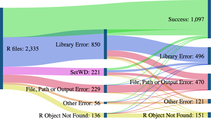
Success rate and errors before and after code cleaning. To objectively determine the effects of code cleaning, we subset the results that have explicit “successes” and errors while excluding the ones with TLE values as the outcome. As a result, the count of files in this figure is lower than the total count.
Most code files had other, more complex errors after code cleaning resolved the initial ones. For example, other library errors appeared if a library was not installed or was incompatible due to its version. Such an outcome demonstrates the need to capture the R software and dependency versions required for reuse. File, path, and output errors often appeared if the directory structure was inaccurate or if the output file was not saved. “R object not found” error occurs when using a variable that does not exist. While it is hard to pin the cause of this error precisely, it is often related to missing files or incomplete code. Due to the increased success rate with code cleaning, we note that many common errors could be avoided. There were no cases of code cleaning “breaking” the previously successful code, meaning that a simple code cleaning algorithm, such as this one, can improve code re-execution. Based on our results, we give recommendations in Section 4.
RQ 6. Are code files designed to be independent of each other or part of a workflow?
R files in many datasets are designed to produce output independently of each other (Fig. 9a), while some are structured in a workflow (Fig. 9b), meaning that the files need to be executed in a specific order to produce a result. Due to the wide variety of file naming conventions, we are unable to detect the order in which the files should be executed. As a result, we may run the first step of the workflow last in the worst case, meaning that only one file (the first step) will run successfully in our re-execution study.
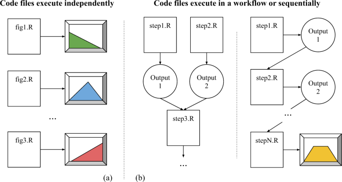
Types of workflows in research analyses.
To examine the nature of R analysis, we aggregate the collected re-execution results in the following fashion. If there are one or more files that successfully re-executed in a dataset, we mark that dataset as’success’. A dataset that only contains errors is marked as’error’, and datasets with TLE values are removed. In these aggregated results (dataset-level), 45% of the datasets (648 out of 1447) have at least one automatically re-executable R file. There is no drastic difference between the file-level success rate (40%) and the dataset-level success rate (45%), suggesting that the majority of files in a dataset are meant to run independently. However, the success rate would likely be better had we known the execution order.
If we exclude all datasets that contain code in other programming languages, the file-level success rate is 38% (out of 2483 files), and the dataset-level success rate is 45% (out of 928 datasets). These ratios are comparable to the ones in the whole dataset (40% on file-level and 45% on dataset-level), meaning that “other code” does not significantly change the re-execution success rate. In other words, we would expect to see a lower success rate if an R file depends on the execution of the code in other languages. Such a result corroborates the assumption that R files were likely designed to be re-executed independently in most cases.
RQ 7. What is the success rate in the datasets belonging to journal Dataverse collections?
More than 80 academic journals have their dedicated data collections within the Harvard Dataverse repository to support data and code sharing as supplementary material to a publication. Most of these journals require or encourage researchers to release their data, code, and other material upon publication to enable research verification and reproducibility. By selecting the datasets linked to a journal, we find a slightly higher than average re-execution rate (42% and aggregated 47% instead of 40% and 45%). We examine the data further to see if a journal data sharing policy influences its re-execution rate.
We survey data sharing policies for a selection of journals and classify them into five categories according to whether data sharing is: encouraged, required, reviewed, verified, or there is no policy. We analyze only the journals with more than 30 datasets in their Dataverse collections. Figure 10 incorporates the survey and the re-execution results. “No-policy” means that journals do not mandate the release of datasets. “Encouraged” means that journals suggest to authors to make their datasets available. “Required” journals mandate that authors make their dataset available. “Reviewed” journals make datasets part of their review process and ensure that it plays a role in the acceptance decision. For example, the journal Political Analysis (PA) provides detailed instruction on what should be made available in a dataset and conducts “completeness reviews” to ensure published datasets meet those requirements. Finally, “verified” means the journals ensure that the datasets enable reproducing the results presented in a paper. For example, the American Journal of Political Science (AJPS) requires authors to provide all the research material necessary to support the paper claims. Upon acceptance, the research material submitted by authors is verified to ensure that they produce the reported results20,21. From Fig. 10 we see that the journals with the strictest policies (Political Science Research and Methods, AJPS, and PA) have the highest re-execution rates (Fig. 10a shows aggregated result per dataset, and Fig. 10b shows file-level results). Therefore, our results suggest that the strictness of the data sharing policy is positively correlated to the re-execution rate of code files.

Re-execution success rate per journal Dataverse collection. In the brackets are the number of datasets and the number of R files, respectively.
RQ 8. How do release dates of R and datasets impact the re-execution rate?
The datasets in our study were published from 2010 to July 2020 (Table 2), which gives us a unique perspective in exploring how the passing of time affects the code. In particular, R libraries are not often developed with backward compatibility, meaning that using a different version from the one used originally might cause errors when re-executing the code. Furthermore, in some cases, the R software might not be compatible with some versions of the libraries.
Considering the release years of R versions (Table 3), we examine the correlation in the success rates between them and the release year of the replication package. We find that R 3.2, released in 2015, performed best with the replication packages released in 2016 and 2017 (Fig. 11a). Such a result is expected because these replication packages were likely developed in 2015, 2016, and 2017 when R 3.2 was frequently used. We also see that it has had a lower success rate in recent years. We observe that R 3.6 has the highest success rate per year (Fig. 11b). This R version likely had some backward compatibility with older R subversions, which explains its high success rate in 2016 and 2017. Lastly, R 4.0 is a recent version representing a significant change in the software, which explains its generally low success rate (Fig. 11c). Because R 4.0 was released in summer 2020, likely none of the examined replication packages originally used that version of the software. It is important to note that the subversion R 3.6 was the last before the R 4.0 (i.e., there was no R 3.7 or later subversions). All in all, though we see some evidence of backward compatibility, we do not find a significant correlation between the R version and the release year of a replication package. A potential cause may be the use of incompatible library versions in our re-execution step as the R software automatically installs the latest version of a library. In any case, our result highlights that the execution environment evolves over time and that additional effort is needed to ensure that one can successfully recreate it for reuse.

Re-execution success rates per year per R software version.
Looking at the combined result from Fig. 11d, we are unable to draw significant conclusions on whether the old code had more or fewer errors compared to the recent code (especially considering the sample size per year). Similarly, from 2015 to 2020, we do not observe significant changes in the dataset size, the number of files in the dataset, nor the number of R code files, which remain around reported values (see RQ 1). However, we see that the datasets use an increasing number of (unique) libraries over time, i.e., from an average of 6 in 2015 to about 9 in 2020.
RQ 9. What is the success rate per research field?
The Harvard Dataverse repository was initially geared toward social science, but it has since become a multi-disciplinary research data repository. Still, most of the datasets are labeled’social science,’ though some have multiple subject labels. To avoid sorting the same dataset into multiple fields, if a dataset was labeled both “social science” and “law,” we would keep only the latter. In other words, we favored a more specific field (such as “law”) and chose it over a general one (like “social science”) when that was possible.
The re-execution rates per field of study are shown in Fig. 12. The highest re-execution rates were observed for the health and life sciences. It may be that medical-related fields have a stronger level of proof embedded in their research culture. Physics had the lowest re-execution rate, though due to the low sample size and the fact that Dataverse is probably not the repository of choice in physics, we cannot draw conclusions about the field. Similarly, we cannot draw conclusions for many of the other fields due to the low sample size (see the number of R files in the brackets), and therefore, the results should not be generalized.
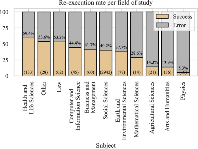
Success rate per research field.
RQ 10. How does the re-execution rate relate to research reproducibility?
Research is reproducible if the shared data and code produce the same output as the reported one. Code re-execution is one of the essential aspects of its quality and a prerequisite for computational reproducibility. However, even when the code re-executes successfully in our study, it does not mean that it produced the reported results. To access how the code re-execution relates to research reproducibility, we select a random sample of three datasets where all files were executed successfully and attempt to compare its outputs to the reported ones. There are 127 datasets where all R files re-executed with success (Table 4).
The first dataset from the random sample is a replication package linked to a published paper at the Journal of Experimental Political Science22. It contains three R files and a Readme, among other files. The Readme explains that each of the R files represents a separate study and that the code logs are available within the dataset. Comparing the logs before and after code re-execution would be a good indication of its success. After re-executing two of the R files, we find that the log files are almost identical and contain identical tables. The recreated third log file nearly matched the original, but there were occasional discrepancies in some of the decimal digits (though the outputs were in the same order of magnitude). Re-executing the third R file produced a warning that the library SDMTools is not available for R 3.6, which may have caused the discrepancy.
The second dataset from the random sample is a replication package linked to a paper published at Research & Politics23. It has a single R file and a Readme explaining that the script produces a correlation plot. According to our results, it should be re-executed with R 3.2. The R file prints two correlation coefficients, but it is unable to save the plot in the Docker container.
The final dataset from our sample follows a paper published at the Review of Economics and Statistics24. It contains two R files and a Readme. One of the R files contains only functions, while the other calls the functions file. Running the main R file prints a series of numbers, which are estimates and probabilities specified in the document. However, the pop-up plotting functions are suppressed due to the re-execution in the Docker container. The code does not give errors or warnings.
While successful code re-execution is not a sufficient measure for reproducibility, our sample suggests that it might be a good indicator that computational reproducibility will be successful.